
Table of contents
The “Inside the machine” series by Giuseppe Ciuni continues. In the first article, we looked at what an LLM is — a statistical text simulator that predicts the next token — along with tokenisers, RAG and the first business use cases. In the second article, we looked at how a neural network learns: loss, gradient, learning rate, Adam and autograd. This third article answers the question that remained open: what exactly does the model operate on? Not on words. On vectors.
The concepts that will be introduced in this article are as follows:
- Embedding (the vector representation of tokens)
- Positional encoding (how the model knows the order of the words)
- Self-attention (how the model connects tokens to one another)
- Multi-head attention (multiple parallel readings of the same text)
Each of these concepts explains a specific behaviour of the model in production. A CTO or founder integrating AI into their company will sooner or later have to answer questions such as these:
- Why does a model that performs excellently in English perform less well in Italian, or when it comes to technical industry terminology?
- Why does extending the scope cause costs to skyrocket?
- Why does the model itself recognise that the ‘football’ played in a match and the ‘football’ that’s good for your bones are two different things?
Let’s take it one step at a time, as always.
Picking up from the previous article
In Article 2, we left the model in training: the loss measures the error, the gradient indicates the direction of correction, and Adam adjusts the parameters step by step. But one question remains unanswered: what is the neural network processing?
What about tokens as integers? No, and understanding why is the starting point.
Let’s recap what a tokeniser does (we introduced it in Article 1): it breaks the text down into pieces – tokens – and assigns a number to each piece, drawing it from a fixed vocabulary.
It’s like a huge dictionary in which every entry has a number: ‘cat’ is entry number 4821, ‘pizza’ is 4822, ‘feline’ is 7980, and so on.
After passing through the tokeniser, the text no longer consists of words but of a sequence of these numbers, as shown in the figure below:
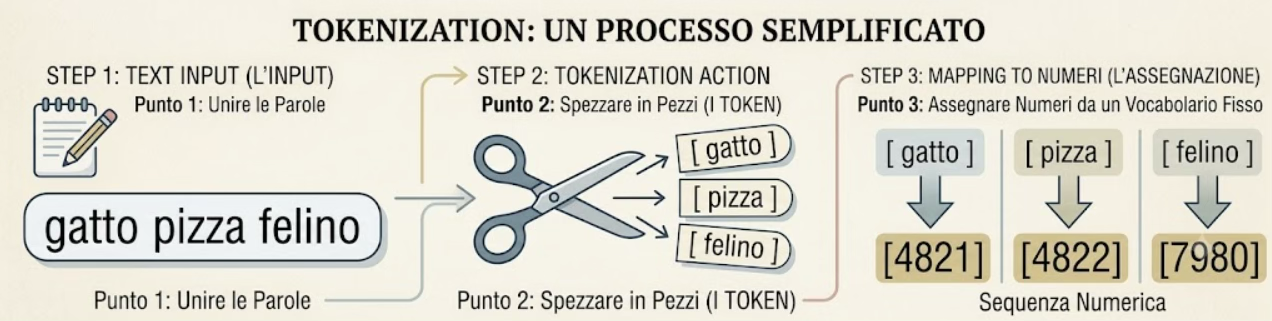
Figure 1. The tokeniser in three steps: it takes the text, breaks it into pieces (the tokens) and assigns each one a number from a fixed vocabulary. The result is a sequence of numbers in place of the words.
The problem is that that number is just a label, not a measure. It’s like a footballer’s shirt number: it serves to identify him, but it says nothing about what sort of player he is. The number 10 and number 11 shirts are close together, but that doesn’t mean the two players are alike.
The same applies to tokens.
“Cat” (4821) and “pizza” (4822) have consecutive numbers but have nothing to do with one another: they happen to be next to each other purely by chance, like two words that are adjacent in alphabetical order.
Conversely, ‘cat’ (4821) and ‘feline’ (7980) are very closely related concepts, but their numbers are very far apart; see the example in Figure 2.
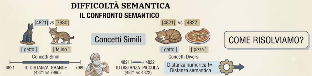
Figure 2: The numerical distance between tokens says nothing about their meaning: ‘cat’ (4821) and ‘feline’ (7980) are semantically close but numerically far apart, whilst ‘cat’ (4821) and ‘pizza’ (4822) have almost identical numerical values but are different concepts
In other words: the distance between the numbers bears no relation to the distance between the meanings. The index (the number) identifies the token but carries no information about what that token means.
A neural network works by calculating distances, sums and relationships between numbers. Given what we’ve discussed, we need a more sophisticated conversion that transforms each token into something that truly encodes its meaning.
That conversion is called embedding.
Embedding
Once a token has been converted into an index by the tokeniser, it is transformed into a vector: a list of numbers in a high-dimensional space.
In modern models, this dimension typically has a value of 768, 1,024 or even 4,096 (OpenAI’s text-embedding-ada-002 algorithm, for example, uses 1,536).
The fundamental property of these vectors is not their dimension: it is their geometry.
During training, the model learns to place tokens in this space so that tokens with similar meanings are placed close together. This is not a manual decision made by a programmer: it emerges automatically from the gradient during training. The result is a sort of geographical map of the language.
In fact, words with similar semantic relationships form clusters: “King”, “Queen” and “Prince” end up grouped together; “Cat”, “Dog” and “Feline” form another group.
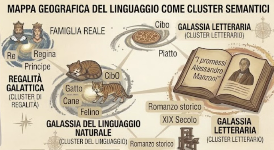
Figure 3: The similarity clusters are shown: the cat, the dog and the feline belong to one cluster. The historical novel *The Betrothed*, published by Gutenberg, belongs to another cluster.
One interesting thing about vectors is that proximity isn’t limited to synonyms: in a well-constructed space, the vector for the phrase “Quel ramo del lago di Como” ends up close to those for “I promessi sposi” and “Alessandro Manzoni” because they appear in the same contexts within the texts.
This structure has a direct practical implication. When you ask a model, “Which places would you recommend I visit in Sicily?”, not only are the words of the question converted into vectors, but the model also “knows” which vectors are close to “Sicily” and uses that context to construct its response.
Finally, there is a surprising property: semantic relations are preserved as vector operations. The relation “King − Man + Woman” in the embedding space produces a vector close to “Queen”. (This brings us back to the vector spaces and linear algebra we studied in Geometry!)
It’s not a trick: it’s an emergent property of training on large corpora.
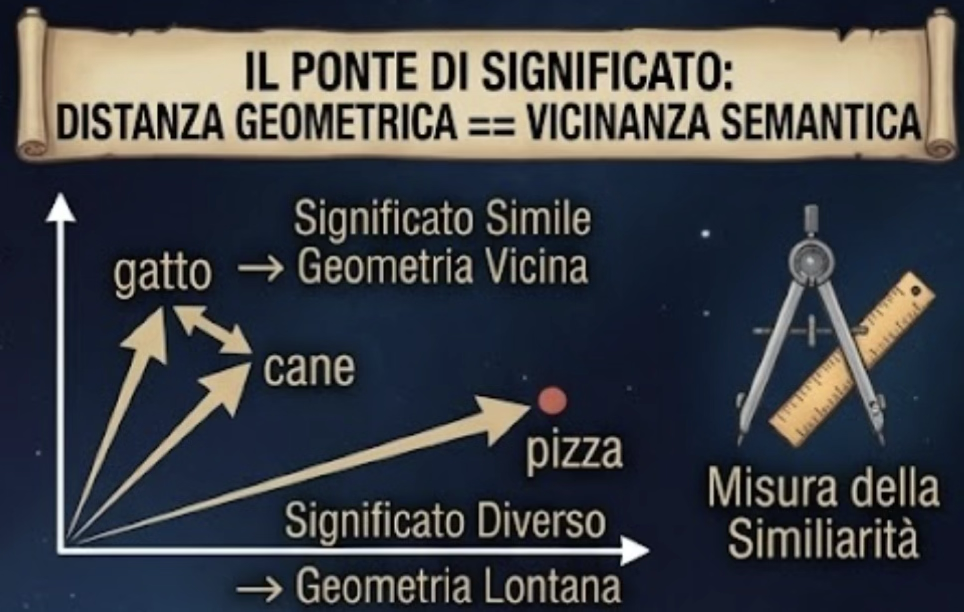
Figure 4: 2D projection of the embedding space — semantic clusters
What exactly are these vectors?
A vector is simply a list of numbers: think of it as a fact sheet for a word. Just as a person’s profile contains lots of different details (age, height, town, job, hobbies), a token’s profile contains lots of numbers, and each one describes a small aspect of its meaning.
And here you can see what the 1,024 dimensions are for: they are simply 1,024 cells, 1,024 numbers for each word.
Why so many? Because a single number wouldn’t be enough to convey the meaning.
If I had only one piece of information to describe a person (let’s say their height), two people of the same height would appear identical even though they are very different. By adding age, occupation, interests and city, however, I can determine much more precisely how similar or different two people are.
The same applies to words: with 1,024 values, the model can capture 1,024 different nuances, so two words may be similar in some respects and quite different in others. An important point: these cells do not have labels that we have decided on (there is no cell labelled ‘it is an animal’ or ‘it is positive’); it is the model itself that decides what to put in them.
The question remains: we have the labels for the boxes, but who fills in the values for the actual boxes?
None by hand.
At first, they are filled with random numbers, so each word starts at a random point on the map, making no sense. Then the mechanism of Article 2 kicks in.
The model makes a guess, gets it wrong, and measures how far off it was (the loss). This is where backpropagation comes into play. Put simply, it is the process by which the model starts from the final error and works its way back through all the calculations it has made to work out how much each number contributed to the error. Once it has worked this out, it adjusts each number slightly, in the direction that minimises the error. By repeating this process thousands of times, words that appear in similar contexts end up moving closer together on the map.
The geometry is not designed but emerges from this continuous adjustment.
That’s why it’s said that embeddings are model weights just like any others: the cells for each word are numbers that the training process adjusts in exactly the same way as it does for the rest of the network. They’re just the first ones to be created, and there are loads of them!
Let’s take an example: 50,000 words, each with 1,024 cells, gives 50,000 × 1,024 ≈ 51 million numbers. This table is, quite literally, the embedding matrix: one row per word, one column per dimension (see table below).
51 million parameters used just to describe the words before even building the rest of the model: that explains the staggering figure of 3B parameters for one model, 11B for another, and so on. Ah. B stands for billion.
Let’s take an example of embedding the words ‘dog’, ‘cat’ and ‘hammer’, simplifying the dimensions to 6 (rather than 1024).
| Is he alive? | Is it domestic? | Is it big? | related to food? | Is it emotional? | Is it an object? | |
| Cat | 0,9 | 0,8 | −0,6 | 0,1 | 0,7 | −0,9 |
| Dog | 0,9 | 0,8 | 0,1 | 0,1 | 0,8 | −0,9 |
| hammer | −0,9 | −0,8 | −0,2 | −0,3 | 0,0 | 0,9 |
Read as it stands, the “cat” entry reads:
- very much alive (0.9)
- very domestic (0.8)
- rather small (−0.6)
- not particularly related to food (0.1)
- emotional (0.7)
- is not an object (−0.9)
If we compare dogs with cats, we have:
“Dog” has almost the same number of occurrences as “cat”: that’s why they end up close to each other on the map.
“Martello” has almost opposite scores for “living” and “object”: that is why it ends up far away. This means that similar words have similar vectors: they have lists of similar numbers.
In microgpt, Karpathy’s 200-line GPT, everything is stripped down to the bare essentials: the tokeniser processes characters one by one, and the vocabulary consists of the 26 letters of the alphabet plus a special token that marks the start and end of each word (27 tokens in total). Each token becomes a vector of just 16 dimensions. The entire model has around 4,000 parameters. It is precisely this miniaturisation that makes it readable in an afternoon: the embedding matrix is the first thing to be initialised, and each row corresponds to a token, each column to a dimension of the semantic space.
The difference compared to GPT-4 is in the order of magnitude of the numbers, but the structure is identical.
Positional encoding
There is one problem that embeddings alone cannot solve: the network does not know the order in which the words arrive. The way it is designed, it receives the word vectors all at once, as if they had been thrown into a bag. A bag has no order!
The point is that the order changes everything. “The cat eats the mouse” and “The mouse eats the cat” contain exactly the same words but mean the opposite. If the network only sees the set of words, it treats the two sentences as identical, and that’s not right.
The solution is called positional encoding.
The idea is simple: before feeding the words into the network, information about where each word appears in the sentence is attached to it. In effect, in addition to the vector that identifies the word (the embedding), a second vector is added that indicates its position. Thus, the same word ‘cat’ receives a different signal depending on whether it is the first word in the sentence or the seventh.
Conceptually, it is a sum:
final_word = word_vector + position_vector.
The two vectors are added together to form a single vector, which is the one that actually enters the network.
One final note on microgpt: in keeping with the GPT-2 style, positions are not calculated using a fixed formula. These are values that the model learns on its own during training, in exactly the same way as it learns embeddings.
In other words, it is the model itself that determines the most useful way to represent the ‘first’, ‘second’, ‘third’ word and so on.
Self-attention
Embedding and positional encoding address the representation of individual words. The most difficult problem remains: context.
Let’s consider the word “pesca”. In “I ate a peach”, it is a fruit; in “I went fishing”, it is an activity. As you can see, “pesca” is the same token, so it starts with exactly the same embedding. The correct meaning can only emerge by looking at the other words in the sentence. This is precisely the problem that self-attention solves: for each word, it decides which other words to pay attention to in order to clarify its meaning in that context.
The mechanism. Starting from its embedding, each word generates three vectors. How? By multiplying the embedding by three different weight matrices, which are learnt during training just like everything else (for those who want to get technical: in Karpathy’s code, these are called wq, wk and wv).
The three vectors can be interpreted as three roles:
- Query (Q): “What am I looking for to understand myself?” For “fishing” in our sentence: “Is there a verb of movement nearby, or a word related to food?”
- Key (K): “What kind of word am I? What do I offer others?” The “past tense” label says: “I am a verb of motion”.
- Value (V): “If they pay attention to me, what message am I conveying?”. The content of “past”: the idea of action, of movement.
A metaphor might help: a fair!
Each participant takes turns with:
- a question on my mind (the query)
- a badge on their chest that says who they are (the key)
- a folder containing the materials to be handed in (the value)
Everyone stops at the desks whose badges match their query — and takes the materials from those desks, and only from those.
We organised one a while back, and watching how people behaved, that’s exactly what it was: people asking questions, wearing a name badge on their chest and carrying a folder full of various materials.
From here, the process takes place in three steps.
1. How well two words go together. Take the “query” from the first word and the “key” from the second; as both are numbers, multiply them digit by digit and add the results together.
This results in a single number: the more the two lists resemble each other, the higher that number is. The cell-by-cell multiplication rewards pairs that have high values in the same places, i.e. that ‘talk about the same things’. This number is the attention score between the two words.
2. From scores to percentages. The scores obtained in this way are converted into percentages which, when added together across all the words, total 100% (this is done by a function called softmax). In this way, for each word, we know how much weight to assign to each of the others: for example, 70% to one, 20% to another, and 10% to a third.
3. The text is updated. Each word incorporates some of the ‘content’ of the others (the Value), taking on as much as its percentage of attention dictates. A word that has received 70% carries significant weight, whilst one that has received 10% carries almost none. The result is a new vector for that word, enriched by its surroundings.
Let’s look at an example with numbers. Let’s stick with “I went fishing” and put ourselves in the shoes of “fishing”, which has to work out whether it refers to the fruit or the activity.
For simplicity’s sake, let’s look at just two of the neighbouring words, “andato” and “a”, and use six cells: “pesca” displays its query, the others display their labels (the keys).
| c1 | c2 | c3 | c4 | c5 | c6 | |
| “Fishing” query | 0,9 | 0,1 | 0,0 | 0,8 | 0,2 | 0,1 |
| “Out” key | 0,8 | 0,0 | 0,1 | 0,9 | 0,1 | 0,0 |
| Key “a” | 0,1 | 0,2 | 0,1 | 0,0 | 0,1 | 0,2 |
Columns c1–c6 are the elements of the vector: numbered positions that do not have a meaning that is immediately clear to a human being. To simplify matters and illustrate the concept, c1 = ‘how much I am a verb’, c2 = ‘how much I talk about food’, and so on. In effect, it is a vector that represents the geometry of the word.
To see how well “pesca” and “andato” go together, let’s compare their two lines line by line.
The rule is simple: when both of them have a large number in the same square, that square is ‘worth a lot’.
In our case, this occurs in row c1 (0.9 and 0.8) and row c4 (0.8 and 0.9): both rows contain high numbers, so the two words are very closely aligned.
All in all, the score is high: 1.46.
With “a”, however, this never happens: whereas “pesca” has high scores, “a” has low ones. The two words have nothing in common and the score remains low, at around 0.15.
These scores are now converted into attention percentages: since 1.46 is much higher than 0.15, “pesca” receives the lion’s share of its attention (around 75%) and “a” only a fraction (around 10%); the rest is distributed amongst the other words in the sentence.
At this point, ‘pesca’ takes on a new meaning, drawing primarily on the connotations of ‘andato’, which is a verb denoting movement. Thus, ‘pesca’ takes on a sense of action, and its meaning shifts towards the activity (going fishing) rather than the fruit.
In other words, she might have overheard different neighbours and ended up on the side of the fruit. The context did its job.
The metaphor. Let’s think about how we read. When we come across an ambiguous word, our eyes briefly go back to the surrounding words to clarify its meaning. When reading “I went fishing”, it is “went” that tells us what kind of fishing it is, not “to”.
Self-attention does exactly that: each word ‘re-reads’ the others in the sentence, focusing on those that help it to understand itself and ignoring the rest.
Let’s look at a visual example to make it clearer. Below is the attention matrix for the sentence “I went fishing”
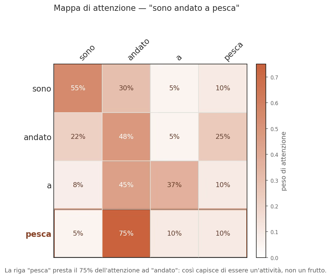
Figure 5: Attention matrix for “I went fishing”: each row shows how much attention a word pays to the others (total 100%). The “fishing” row pays 75% of its attention to “went”, and this is why it understands that it is an activity, not a fruit.
How to read this matrix in three steps:
- Lines are words ‘that look’. Choose a row: it is a word in the sentence as you try to make sense of it. The grid has four rows because the sentence has four words: “sono”, “andato”, “a”, “pesca”.
- The columns represent the words ‘viewed’ in the same order. When you scan a row from left to right, each cell indicates how much attention that word (the row) pays to each other word (the column). The number in the cell is the percentage of attention, and the colour makes this clearer: the darker the colour, the more attention is paid.
- Each row totals 100%. The focus of a word is a ‘cake’ shared out among all the others.
The focus of the diagram is the bottom row: “pesca” (highlighted in dark brown). You can see where the focus lies: 75% on “andato” (the darkest cell), 10% on “a”, 10% on the word itself, and 5% on “sono”.
In practice, the word “pesca” primarily conveys the idea of “going” (a word denoting movement), and it is precisely for this reason that it tends to be associated with the activity of fishing rather than with the fruit.
The famous saying ‘a picture is worth a thousand words’ is true. Looking at the matrix, the following observations emerge:
- the diagonal (sono→sono, andato→andato…) is often highlighted because each word draws a little attention to itself;
- ‘Empty’ words such as ‘a’ receive little attention from others; they are clearer and play a minor role in conveying meaning;
- If the sentence were changed to “I ate a peach”, the word “peach” would be highlighted under “ate” rather than “gone”, and the meaning would shift to refer to the fruit. The map always relates to that particular sentence.
Multi-head attention
A single self-attention operation captures one type of relationship at a time. But in a sentence, there are many relationships, all occurring simultaneously: grammatical relationships (who is the subject, who is the verb), relationships of meaning, relationships of reference (who is referred to by ‘it’ or ‘this’), and temporal relationships.
A single “reading” is not enough to grasp everything.
Multi-head attention solves this problem by performing multiple parallel passes rather than a single one. Each pass is a complete self-attention mechanism with its own Query, Key and Value, and can choose to specialise in a different type of relationship. Each pass is called a ‘head’.
To give an idea of the scale: GPT-2 Small has 12 heads, whilst GPT-4 is estimated to have hundreds. In MicroGPT, for simplicity’s sake, there are four on a single attention layer.
To return to the earlier example: it is like reading the same sentence over and over again, but each time looking for something different: one reading follows the grammatical structure, another the cause-and-effect relationships, and yet another works out which words the pronouns refer to.
In the end, all these readings are combined into a single result.
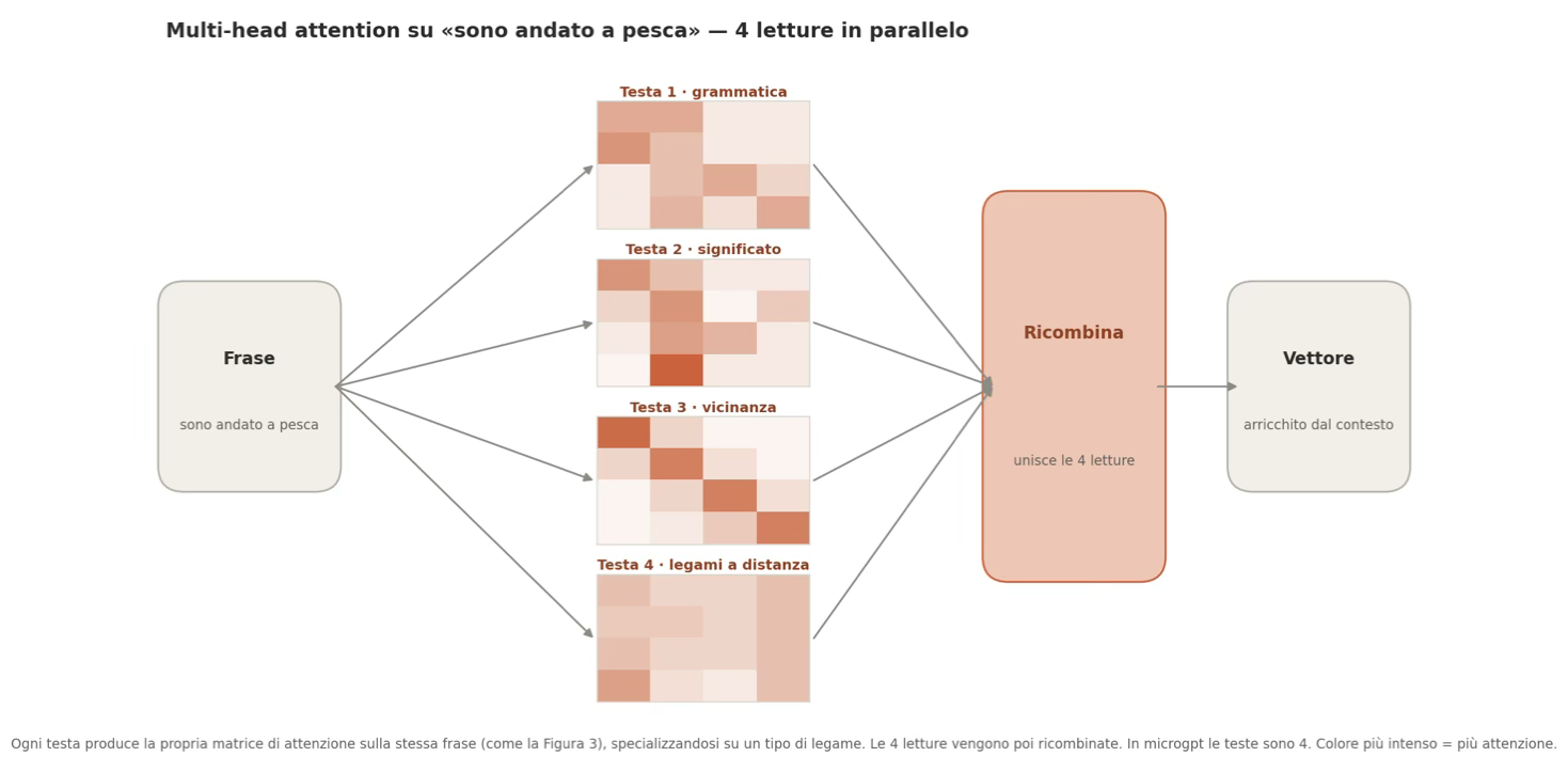
Figure 6: Multi-head attention architecture with multiple heads operating in parallel to produce a recombined output
The result of all this is a new vector for each word, enriched by the context of the entire sentence. No longer a fixed point on the map of language, but a point that has shifted according to its surroundings.
What is a transformer?
We have just looked at two mechanisms: self-attention, whereby each word ‘looks’ at the others in the sentence and absorbs their context (this is how ‘pesca’ in ‘sono andato a pesca’ understands that it refers to an activity and not a fruit), and multi-head attention, which repeats that same process several times in parallel to identify different connections. This set of operations is known as a Transformer.
Transformer is the name of the architecture – that is, the framework that brings together all the elements we have seen so far in the correct order:
- embedding
- positional encoding
- attention (self-attention and multi-head)
In fact, this is the architecture on which all modern models are based, from GPT to Claude to Gemini. The ‘T’ in GPT stands for Transformer.
It originated in 2017 from a now-famous Google article, “Attention is all you need”: the idea, which was revolutionary at the time, was that attention alone was enough to understand language.
The transformer consists of a block that repeats itself identically.
Within each block, two things happen one after the other: first, the words exchange information with the attention, then each one processes what it has gathered on its own (this is the feed-forward at the bottom).
The power of these models lies in lining up many of these blocks, one on top of the other. ‘Stacking’ means connecting them in sequence: the output from the first block goes into the second, the output from the second goes into the third, and so on. Each block processes the result already refined by the previous one and improves it a little further.
Let’s look at our usual example, “I went fishing”, focusing on the word “fishing”, which is somewhat ambiguous.
As we have seen in the matrix, in the first section her focus makes her look primarily at the past tense, and by the time she reaches ‘pesca’, her focus has already shifted to the meaning of the activity.
This concept, now clearer, moves on to the second section, which further refines it: for example, it recognises that ‘andato a pesca’ is a single expression, a way of saying ‘to go fishing’.
Block by block, the meaning becomes clearer and clearer. That’s why the number of blocks matters!
The block structure is always the same; the only thing that changes is how many are stacked: just one in microgpt, 12 in GPT-2 small, and several dozen in state-of-the-art models.
The more blocks a word passes through, the better the model is able to capture nuances and, therefore, the better it ‘understands the meaning of what we write’.
Microgpt has just one block, perhaps for the sake of readability (in my opinion). I’m tempted to use an expression from my dialect to say: I wonder how many blocks Anthropic uses in Fable 5.
The other components of the block
To really understand Karpathy’s code, you need three more ingredients, which, along with attention, complete the picture. They are less well-known, but without them the model would not train.
A useful tip before you start: a neural network works in stages, like an assembly line, and each stage is called a layer.
Here are the ingredients:
Feed-forward. After ‘listening’ to its neighbours, each neuron processes the information it has gathered on its own, as if returning to its desk. Its vector is expanded (in microgpt from 16 to 64 numbers) and then compressed again. In between, ReLU comes into play, an algorithm that removes negative numbers: it keeps the positive ones as they are and sets the negative ones to zero. This small rule gives the calculation a “bend” which serves to distinguish one layer from another so that they can be stacked, allowing the network to grasp complex relationships.
Residual connection. The result of each step does not replace the initial vector: it is added to it (x = x + correction) as a side note rather than rewriting the whole thing. This is what allows dozens of layers to be stacked without the information (the gradient of Article 2) being lost along the way.
Normalisation. Before each block, the numbers are scaled to a standard range. Without this, they would increase or decrease layer by layer, making the training unstable.
Embedding, Attention, Feed-forward, Residual connections and Normalisation: this is the complete transformer architecture, the building blocks that, when stacked one on top of the other, form the models.
To sum up
- Tokeniser: splits the text and assigns a label number to each word (it identifies the word, but does not indicate its meaning).
- Embedding: transforms that number into meaning by placing the word on the ‘language map’, where similar words are grouped together.
- Positional encoding: it takes into account word order, so “the cat eats the mouse” is different from “the mouse eats the cat”.
- Self-attention: each word takes account of the others and adapts to the context: this is how “pesca” knows whether it refers to a fruit or an activity.
- Multi-head attention: the same self-attention mechanism repeated multiple times in parallel to capture multiple types of connections simultaneously.
- Feed-forward, residual and normalisation: these complete the block, processing the information gathered by the attention mechanism and ensuring the calculations remain stable. They are the traffic controllers☺
Conclusions
In Article 2, we saw how the model learns; in this one, we have discovered what it actually works on: not on words, not on simple numbers used as labels, but on vectors – that is, lists of numbers that assign each word a position on a ‘language map’.
This map isn’t drawn by a programmer: the model builds it itself during training by grouping together words with similar meanings.
The position of a word is not fixed; instead, it is adjusted each time, depending on the context. In this way, ‘pesca’ can refer to the fruit or the activity, depending on the surrounding words.
Tip 1: Vertical fine-tuning starts with the embeddings
When a general-purpose model performs poorly on domain-specific terminology (e.g. legal, manufacturing, medical, financial), the problem often lies in the embeddings. Terms such as ‘anti-decubitus bed’, ‘compound pelvic fracture’ and ‘renal failure’ were rare or absent in the pre-training data: their vectors are positioned almost at random and far from the clusters where they should be.
Fine-tuning using domain data corrects this geometry.
Before purchasing a ‘pre-fine-tuned’ vertical model, it is advisable to ask the supplier what data it was trained on and using which method. If the answers are vague, the fine-tuning has probably not been carried out, or has not been done properly.
Tip 2: A large context window does not necessarily mean a better model
Suppliers are promoting ever-wider context windows as if they were a straightforward advantage.
Self-attention scales quadratically with the length of the sequence: doubling the context quadruples the computational cost for each call. For enterprise applications such as on-premises helpdesks, document classification or contract extraction, 4,000–8,000 tokens are sufficient.
Choosing a model with a context window of 128,000 tokens for tasks of this kind means paying a high price without reaping any benefits. The optimal context window is a parameter that should be measured against real-world tasks, not maximised indiscriminately.
News from a couple of days ago: Autonomous Recursive Improvement – AI rewrites its own code. Source: Anthropic.
Anthropic states that over 80% of the code in its codebase was written by Claude to a standard comparable to that of a human. Individual engineers’ productivity (measured in lines of code) has increased eightfold compared to 2024.
In the next and final issue of Inside the Machine, we’ll bring our exploration of microgpt full circle. We’ll see how the enriched vector becomes a probability ranking and how the model generates text one piece at a time. We’ll understand why output tokens cost more than input tokens, what really controls the ‘temperature’, and what the difference is between the base model and the instruct model, with the two steps that separate them: SFT and RLHF (photo by Igor Omilaev on Unsplash).
ALL RIGHTS RESERVED ©
